Episodic Master Recession techniques to evaluate hydrographs for aquifer recharge and streamflow

Using the EMR Program
The program requires three time series that are in the user's input file plus a forth that is calculated by the program:
- Time, T (as a numerical quantity, e.g. in days)
- Water table level or discharge, R
- Cumulative precipitation, P
- Response rate of change, dR/dT (calculated by the program)
The three time series to be supplied by the user are the same as those needed for MRCfit, so identical input files can be used for the two programs.
The user chooses the time units for use with T and the length units for use with R and P. The same chosen units are used throughout the calculations and output.
There are 4 necessary files: a start file, the main program file, the plotting program, and the input file containing columns of T, R, and P.
Start file: This file contains information that informs the main program such as the location of the main program file, the data file, and the adjustable parameter values.
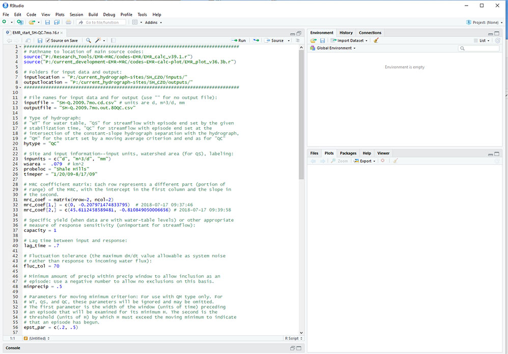
Below is a screen shot of an EMRstart code on the R Studio interface. Lines that require changes are listed below. The # symbol indicates a comment
in the program

- Line 3: Path to the location of the main program file
- Line 4: Path to the location of the main program file
- Line 7: Path to input files
- Line 8: Path to output files
- Line 12: Input data file name
- Line 13: Output data file name (use "" if no output file is desired)
- Line 20: Hydrograph type (WT, QS, QC, or QM)
- Line 23: Units of input (time, response variable, precip)
- Line 24: Watershed area (L^3)
- Line 25: Site, well name, or stream name to appear on graph output
- Line 26: Date to appear on graph output
- Line 32 & 33: MRC coefficients of the polynomial fit to the water level recession data. If only one part fit is used, both lines with have the same values.
- Line 37: Specific yield (value = 1 for streamflow)
- Line 40: Lag time (the typical time difference between the start of rainfall and the first significant change in water level)
- Line 44: Fluctuation tolerance (the maximum dR/dt value allowable as system noise without being considered as episodic recharge)
- Line 48: Minimum amout of precip to start an episode
- Line 56: Episode start param
- Line 62: Episode end param
- Line 67: Moving-average interval used to smooth data
- Line 70: Axis limits for time on graph
- Line 71: Axis limits for response variable on graph
- Line 72: Axis limits for precip on graph
- Line 73: Axis limits for derivative on graph
- Line 79: Units for precip output
- Line 80: Units for rate output
- Line 81: Units for volume output
- Line 85-88: Units needed for converting input units to desired output units. For example, if precip data are in inches and you want the output in mm you would put on a value of 25.4 on line 85.
Main program file (EMR_main_v39.0 or later): this is the main code that takes the input data and determines periods of recharge based on parameters and tolerances set in the start file.
Step by Step Instructions
- Open the RStudio Software
- Go to File -> Open -> Choose your start file
- Insert proper information on lines as described above
- Save the start file
- Click on the "source" button just above the interface file to run the main program (a shortcut useful for trial-and-error procedures is to check the Source on Save box)
Output
- Graph of water levels vs time with recharge periods highlighted
- Graph of water level derivative vs. time with tolerance band recharge periods highlighted
- Output file (.csv format) with quantities of interest. Output files are different for water level and streamflow.
- Additionally, there is another file with a .aux extension that is useful for debugging the code but is generally not used.
Below these values there are columns with infomration on the intervals between episodes which are useful for refining parameter values and evaluating model performance:
A. Nonepisode- just the episode number
B. Start time- start of the episode
C. End time- end of the episode
D. Duration- length of the episode
E. Start input time- precip start time
F. End input time- precip end time
G. End input time- precip end time
H. Water input- precip total for episode
I. Input rate average- average rate for the episode
Columns in output file for streamflow hydrographs:
A. Episode- just the episode number
B. Time since the last episode
C. Start time- start of the episode
D. End time- end of the episode
E. Duration- length of the episode
F. Peak time- time from episode start to the peak response
G. Start response- discharge at the beginning of the episode
H. End response- discharge at the end of the episode
I. Peak response- discharge at the peak of the episode
J. Start input time- precip start time
K. End input time- precip end time
L. Water input- precip total for episode
M. Input rate average- average rate for the episode
N. Interval input rate max- maximum rate for the episode
O. Delta response peak start- difference in response from the episode start to the peak
P. Delta response peak end- difference in response from the peak to the episode end
Q. Stormflow-
R. Stormflow per area-
S. Ratio to input- the ratio of stormflow and precip
Below these values there are columns with infomration on the intervals between episodes which are useful for refining parameter values and evaluating model performance:
A. Nonepisode- just the episode number
B. Start time- start of the episode
C. End time- end of the episode
D. Duration- length of the episode
E. Start input time- precip start time
F. End input time- precip end time
G. End input time- precip end time
H. Water input- precip total for episode
I. Input rate average- average rate for the episode

For more information contact: UZ Flow Webmaster
Last modified: February 2019

